Dear Jason,
Thank you for the quick, thorough and very helpful reply! I was
just looking through the original paper and also wondered about my
sea-surface salinity pixels being much larger than what is usually
available for SST products. I'll try playing around with window
size but, as you point out, I'm wary of using fewer pixels for the
histogram analysis. I haven't tried Canny Edge yet, since my
impression thus far was this is somewhat out of style for
oceanographic purposes, but will try it as well. The summed
product of all the thinned front images doesn't converge as well,
but that makes sense given your clarification that it is purely
spatially based.
 unthinned, stride=1, summed product
 thinned,
stride=1, summed product
thinned,
stride=1, summed product
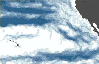
I've attached one of the SSS images to check regarding the
disappearing fronts, as you requested. The image was downloaded
from CP34-BEC, the raster values increased by 100 and then
converted to 16-bit unsigned integer.
Thanks for the help,
Liz
Am 3/9/2016 um 3:57 PM schrieb Jason
Roberts:
Dear
Liz,
Thanks
for your interest in MGET and for including all of the
details of your experiment. Yes, I do believe the
horizontal artifacts you are seeing result from the
16-cell stride used by default in the algorithm. I have
had similar problems as you in trying to apply the
algorithm to various datasets.
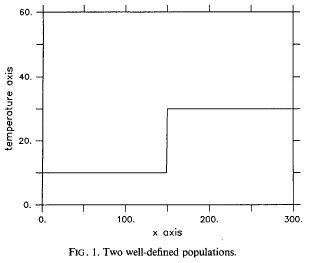
The
core problem is that the algorithm assumes, under ideal
conditions, that 1) there are only two populations in the
moving window (e.g. cold and warm, or salty and fresh),
and 2) each population is composed of constant values (the
same temperature, salinity, etc.). From the 1992 paper:
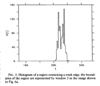
To
detect fronts, the algorithm first tries to determine if
two populations are present. It constructs a histogram of
the cells in the moving window and runs some statistics to
see whether there is a sufficiently bimodal distribution.
In an easy real-world case, the histogram might look like
this:
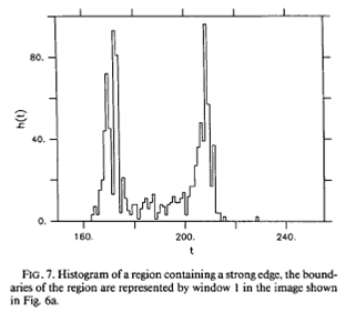
You
can see two clear peaks. In a harder case, it might look
like this:
The
1992 paper was applied to SST data with a cell size of
1.0-1.5km. With that kind of data, particularly in the
area of North Carolina where the Gulf Stream separates
from the shelf of North America, it is easy to satisfy
those two assumptions for windows that are 32x32 pixels.
When coarser data are used, it is harder for those
assumptions to hold for a 32x32 window. As the window
expands to cover a larger geographic area, it might
encompass multiple water masses and fronts, leading to a
distribution with three or more modes. The 1992 paper
discusses this (pp. 73-74) and briefly mentions how the
algorithm could be extended to deal with that situation.
But to my knowledge this was never done, and MGET’s
implementation is based on Cayula’s original Fortran code
which assumed a bimodal distribution (i.e. just one front
in the window).
In
my own experience, the assumptions sometimes still hold
when using 4km SST data, but the algorithm starts to break
down. I have sometimes obtained better results with
smaller window sizes. I usually try 20x20 and sometimes
16x16. If you try that, be sure to adjust the minimum
single-population cohesion and minimum global-population
cohesion parameters, as described in their documentation.
This
is a slippery slope, however. With 32x32, the histogram
has 1024 cells to work with, making the statistics
relatively stable. With 16x16, there are only 256 cells
and the statistics are not as reliable. I have not tried
to go below 16x16.
Another
possibility is to reduce the window stride from one half
the window size (16-cell stride for a 32-cell window), as
you have done. This can often help, but when fronts are
not present as sharp gradients—i.e. when the second
assumption does not hold very well—then each time the
window moves, the histogram population changes slightly,
and the temperature that is chosen by the algorithm to
separate the two populations also changes slightly. This
temperature identifies the front. When it is slightly
different in overlapping windows, then you get large
“blobs” for fronts, like the green areas in the images you
sent.
To
work around that, you can apply the thinning algorithm,
which you have also done. The thinning algorithm is purely
spatial and does not take the original image values into
account in any way.
I
am not sure why stride=16 would detect the red fronts you
overlaid but stride=1 would not. Could you please send me
that image so I can play around with it?
I
have not had good luck applying this algorithm to 0.25
degree resolution data. This led me to implement the Canny
edge detection algorithm in MGET. Have you tried that? I
had better results with that working on 0.2 degree data
from the GHRSST L4 JPL MUR product.
I
hope this helps,
Jason
From:
[mailto:]
On Behalf Of Liz Atwood
Sent: Wednesday, March 9, 2016 4:33 AM
To:
Subject: [mget-help] Cayula-Cornillon histogram
stride width artifacts
Dear mget developers,
First and foremost, thank you for developing such a
comprehensive tool for the field. I am working on
calculating Cayula-Cornillon fronts for the N Pacific from
various remotely sensed datasets, and I have begun the
endeavour using a SMOS surface salinity product. I've got
the tool up and running with a python script run from ArcMap
10.3 (avoiding the GUI since I'll eventually have quite a
few images to process).
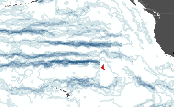
Using the default value histogramWindowStride=16 and then
combining products from 18 different dates (simply summing
them at the moment), one sees that the algorithms is
producing artifacts along what I assume to be the histogram
window edge, notice the horizontal boundaries below (I've
indicated one in red - they come every 16 pixels, darker
blue color indicates pixels where more often a front was
detected).
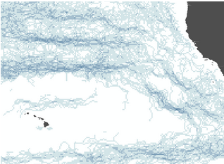
Ok, but I've got a powerful enough computer and so started
experimenting with smaller histogram stride windows. Using a
stride of 1 does not take very long on my system (about 15
seconds) and removed all horizontal boundary artifacts. BUT
some of the fronts now disappear, including before
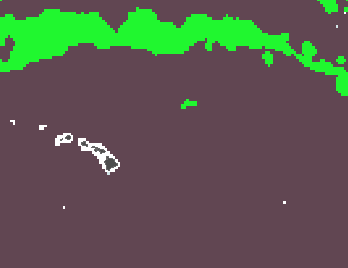
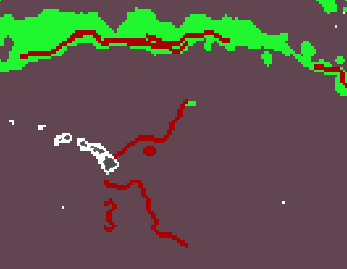
activating the thinning step. The left image is the
unthinned, stride=1 Cayula-Cornillon product for a single
salitiny image (green=1, gray=0). The right image has the
stride=16 product overlaid (in red), where one can see that,
while the northern front is now correctly not being cut-off,
the lower fronts near Hawaii are being detected very
differently.
Any ideas why this would be the case, is there much
experience using a stride=1 or are there other ways to avoid
the horizontal boundary artifacts shown above?
I've included my python script below, if helpful despite its
being pretty basic. Thanks for any help you might be able to
provide.
Best,
Liz
--
Elizabeth C. Atwood
M.Sc. Quantitative Ecology & Resource Management
# this script uses the Cayula-Cornillon algorithm to detect fronts
# for a layer of sea surface salinity images
import arcpy, os, sys
from arcpy import env
from arcpy.sa import *
import GeoEco
from GeoEco import *
import GeoEco.OceanographicAnalysis.Fronts
from GeoEco.OceanographicAnalysis.Fronts import *
mxd = arcpy.mapping.MapDocument("CURRENT")
for lyr in arcpy.mapping.ListLayers(mxd, "BEC_L4_*"):
temp = lyr
tempFile = str(temp)
tName = "D:/Liz/Expedition_Daten/SEA_Law_Pacific/2012/MODIS_A/sss/CayulaCornillonFronts/testing/"+tempFile[0:38]+"_CCfronts.tif"
layer = "D:/Liz/Expedition_Daten/SEA_Law_Pacific/2012/MODIS_A/sss/CayulaCornillonFronts/testing/"+tempFile
# CayulaCornillonEdgeDetection.DetectEdgesInArcGISRaster(layer, 10, tName)
tName2 = "D:/Liz/Expedition_Daten/SEA_Law_Pacific/2012/MODIS_A/sss/CayulaCornillonFronts/testing/"+tempFile[0:38]+"_CCfronts_thin.tif"
CayulaCornillonEdgeDetection.DetectEdgesInArcGISRaster(layer, 30, tName, histogramWindowStride=1)
CayulaCornillonEdgeDetection.DetectEdgesInArcGISRaster(layer, 30, tName2, histogramWindowStride=1, thin=True)